
Info
Purpose of this app
This app is designed to introduce beginner and intermediate R Shiny users to some more advanced concepts, techniques and methods. The initial goal is for this app to serve as a tutorial and cheatsheet for shiny and hopefully introduce R developers in the department to some new shiny solutions and possibilities.
This project will not cover every single thing that R Shiny has to offer. Additionally, although the name implies all topics are at least intermediate level, some are more straightforward and every effort will be made to ensure the content can be understood by those who are fairly new to R Shiny.
A basic knowledge of R and R Shiny is assumed, however. For a beginners introduction to either of these, see the official documentation and get started guide, or check out the Coffee & Coding sharepoint page as there has been previous beginner-level talks on these two topics.
Shiny Ladder of Enlightenment
In a talk at Shiny Dev Con 2016, Joe Cheng (creator of shiny and CTO at RStudio) proposed a (semi-serious) 'Ladder of Enlightenment' for shiny. The ladder gives an idea of different levels of understanding of shiny and how it works (particularly how reactivity works). The ladder is as follows:
- Has used 'output' and 'input'
-
Has used reactive expressions (
reactive()) -
Has used
observe()and/orobserveEvent(). Has written reactive expressions that depend on other reactive expressions. Has usedisolate()properly. -
Can
confidently
say when to use
reactive()vs.observe(). Has usedinvalidateLater(). - Writes higher-order reactives (functions that have reactive expressions as input parameters and return values).
- Understands that reactive expressions are monads.
It is assumed that if you are using this app you are at least at step 1 and probably higher.
Much of the first section of this app, particularly tabs 1.2-1.4 (Understanding, Using and Controlling reactivity) will cover steps 2-4 (and briefly touch on 5).
As Joe commented in his talk, there are probably only a handful of people in the world who are at step 6 (himself and Hadley (Wickham) being two of them). This is because reaching this step would require both expert knowledge of maths and computing, as well as deep understanding of shiny internals and how the package was built. As such this won't be spoken about here. If you're wondering what monads are, I would suggest you don't(!) - if you really want to know you can google 'what are monads' and come back here once you've emerged from the rabbit hole!
Using the app
As you can see, the app has been structured in a similiar fashion to a bookdown site, with sequential chapters that can be accessed using the navigation sidebar. The content has been arranged into three broad categories, which will roughly correspond with the Coffee & Coding sessions to be delivered. The topics are not arranged in order of difficulty, but a logical order has been decided upon and we have tried to put simple or more fundamental concepts earlier on in each section. Feel free to look through each tab in order or to jump around and look at only the parts which interest you.
Where possible, code snippets will be provided which you can copy and paste to try out some of the methods showcased here. The full repository for this app will also be available so you can check out the full code if you want to (link will be provided below at a later date). The app has been structured as an R package (see section 1.5 for more info), so you can clone the repository and run the app yourself with the code below.
remotes::install_github('chrisbrownlie/advancedShiny')
library(advancedShiny)
run_IAS_app()
Note that for any of the code examples which require reactivity, a mini example app will often be provided but if not you can enter a demo reactive state using:
shiny::reactiveConsole(TRUE)
Contributions
This app was developed by:
with contributions from:
For more info or to contribute, contact one of the above.
What Is Shiny?
The Basics
As you are probably aware, shiny is an R package which allows you to build web applications. Although the term 'web application' seems fairly straightforward, it is worth being clear about what this means.
Websites are, at their simplest, a set of files on a computer, which have been made available for other computers to view. They are static, follow certain protocols and always look the same unless the underlying files are explicitly changed. A web app, on the other hand, is a full computer program (application) which can be accessed through a web browser. The benefits of this mean that web apps are far more flexible and dynamic, responding to user actions and rendering pages 'on the fly'. The two terms have more or less become synonymous in recent years, so the vast majority of what we call websites are technically web apps (search engines, social media, news sites etc.).
The front end of most web apps are developed using HTML, Javascript and CSS, as these are supported by pretty much all web browsers. So the short answer to 'What is shiny?', is 'an R to {HTML-Javascript-CSS} translator'. The magic of being able to write R code which gets transformed into a web app written in a completely different language, is what makes shiny so powerful.
A Team Effort (Frameworks)
As well as the package dependencies you can see on the right, shiny also relies on two other frameworks, Bootstrap and jQuery.
Bootstrap
is an 'open source, front-end toolkit' (written in HTML, CSS and Javascript), which lets you build responsive user interfaces quickly
and easily. The Bootstrap repository is the one of the top-10 most starred on Github, which gives some indication as to its popularity. One of the most
common layouts for shiny apps uses the
fluidPage()
,
fluidRow()
, and
column()
functions. All of these -
along with many other shiny UI functions - are simply layered on top of a Bootstrap function (e.g.
fluidPage()
is analogous
to Bootstrap's
bootstrapPage()
function.
jQuery is a javascript package which allows interaction with HTML elements of a webpage, with simpler syntax than pure javascript. This is used to power much of the interactive elements you see in shiny. These are implemented with javascript and jQuery was used to make this process easier.
You can see this for yourself by running a basic shiny app using the code below:
library(shiny)
ui <- fluidPage(p('Hello, world'))
server <- function(input, output) { }
shinyApp(ui, server)
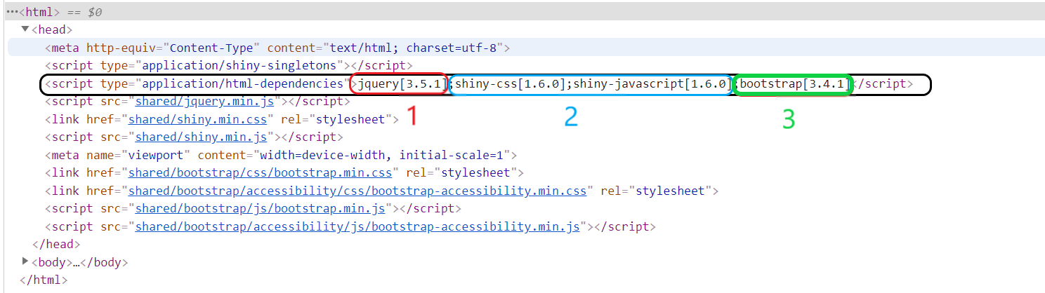
Upon loading the app, open your browsers development tools (on Google Chrome, right click and click 'Inspect'). This will show you the HTML code that shiny has generated for your app. If you open up the header element you can see the dependencies being used (see below), which are:
- jQuery
- shiny (the custom css and javascript elements included in the package)
- Bootstrap 3
Summary
So in summary:
- What shiny does, at its simplest, is translate R code to HTML (and JS and CSS)
- A shiny app uses functionality from 25 other packages too, each addressing their own specific problem
- The most important of these are httpuv, htmltools and jsonlite
- shiny also relies on Bootstrap and jQuery as a minimum
A Team Effort (R Packages)
When you install and use shiny, you are in fact using a collection of separate, interlinked R packages which has shiny at its core. Below you can see which packages are currently imported by shiny and what they do, arranged very roughly (and subjectively) in order of significance:
-
httpuv- Arguably the most important package dependency in terms of how shiny actually works
-
Designed to be used as a 'building block' for R package web frameworks, of which
shinyis the most popular (but not the only, e.g.ambriorixandfieryare alternatives) - Can initiate a web server in R that handles HTTP requests and can also open a websocket (connection between a users computer and the server)
- Essentially does all the heavy lifting when it comes to communication between the client (user) and server
-
htmltools- Perhaps the second most important package for how shiny works, this is used to convert R code into HTML
- If httpuv is the core of a shiny app's server, htmltools is the core of a shiny app's UI
-
jsonlite- Allows the power of Javascript to be utilised in shiny apps by being an R-JS translator
- R and Javascript communicate via websockets (see the box below 'The Lifecycle of a Shiny App') and jsonlite allows this to happen
-
R6- Package for building classes and implementing object-oriented programming in R
- An alternative to built in Reference Classes (RC) in R. R6 is simpler and more efficient so was preferred for shiny
- Most of the fundamental R objects underlying a shiny app are R6 classes (the reactive log, reactive environment, shiny session etc.)
-
cachem- Enables storing of key-value pairs in an on-memory or on-disk cache
- Automatically prunes to make sure memory usage doesn't get too high
- Outputs of reactive objects (e.g. plots) are cached, so that they don't update periodically when inputs remain the same (explained more in the next section 'the reactive graph')
-
rlang- An RStudio package for translation between base R and tidy R. Contains functions for tidy evaluation and improvements on base object types
-
Contains a hashing function that is used whenever a unique ID needs to be assigned to something (e.g the keys for object stored using
cachem -
This hashing was done using the (non-RStudio) package
digest, until shiny v1.7 (Sep 2021) when it was replaced byrlang::hash()
-
bslib: the most recently added dependency, allows usage of Bootstrap 4 (and soon 5) in shiny apps -
later: used to execute code after a set amount of time (e.g. theinvalidateLater()function. Crucially it allows time-specific delays which do not block R from completing other tasks. -
promises: a package for asynchronous programming in R. Since shiny v1.1.0, support was added to reactive elements to allow using promises to speed up apps -
fastmap: an efficiency package, which makes some small improvements to storage of data structures to address the problem of memory leakage that R suffers from -
mime: used to infer a filetype (MIME type) from an extension (i.e. when a user uploads a file) -
withr: a useful package that helps working with functions that have side effect. Includes helpers which mean you can run functions and be sure they will never affect the global environment -
crayon: for outputting messages with coloured, formatted code -
glue: package for concatenating and working with strings -
xtable: used to render tables withrenderTable() -
sourcetools: fast reading and parsing of R code, comparable to readr -
commonmark: used to convert markdown to other formats like HTML and LaTeX, powers theshiny::markdown()function -
ellipsis: used for checking arguments that have been supplied to functions with the ellipsis (e.g. ensure ellipsis arguments are unused if they are just included 'for future expansion') -
grDevices: base R package that allows for controlling of multiple graphics 'devices' - used for rendering plots withrenderPlot() -
lifecyle: used to indicate function lifecycles (e.g. 'experimental', 'maturing', 'deprecated') -
methods,utils,tools: base R packages that respectively: enable S3 and S4 classes; enable various utility functions; and provide tools for package development.
The Lifecycle of a Shiny App
So what actually happens when you run
runApp()? In other words, if you have a deployed shiny
app and someone opens it up (which causes runApp() to be executed), what happens? Well, the following things happen:
-
shiny::shinyApp()is called, which returns a shiny app object composed of a server function and the UI. The UI has to be formatted to be a function returning an HTTP response, as requested by httpuv. -
shiny::startApp()is called, which creates HTTP and websocket (WS) handlers.- To make shiny interactive, R must be able to talk to Javascript and this can be done with traditional HTTP requests.
- However, with a traditional HTTP request model: a connection is opened; the client sends a request; this is processed by the server and a response returned; and then the connection is closed. This is inefficient for this R-JS communication, where there could be hundreds if not thousands of actions to be executed in the course of an app session (and therefore hundreds of connections opened and closed).
- Websockets are an advanced solution to this which allow what is essentially a secure, constant, bi-directional connection between a client and server (Javascript and R).
- This means that over the course of an app session, R and Javascript can communicate quickly and efficiently, passing messages as JSON (which is a format both languages understand).
- The websocket handlers created in this step are responsible for controlling the websocket behaviour after the app starts.
- This step is necessary to allow communication between R and JS.
-
httpuv::startServer()is called, which starts the HTTP server and opens the websocket connection. - If the R code does not contain errors, the server returns the Shiny UI HTML code to the client (user).
- The HTML code is received and interpreted by the client web browser.
- The HTML page is rendered. It is an exact mirror of the initially provided ui.R code
- Any communication between R and Javascript, is formatted as JSON and passed via the established websocket.
Understanding Reactivity
Reactive Programming
Reactive programming is a paradigm that has been around for a while in software engineering and is based on the concept of values which change over time in response to certain actions, and calculations that use these values (and therefore also return different outputs over time). Reactive programming is extremely common and the most widely-used example is a spreadsheet program. In a spreadsheet (e.g. Excel), you define relationships between cells, and if a cell's value gets updated or overwritten then everything that has a relationship with that cell also updates.
In shiny, reactive programming is what makes apps interactive. Users can change values and anything which relies on those values will be recalculated. The power of shiny is in the way it a) implements reactive programming in a language (R) that is inherently not reactive and b) how it determines the optimal way to execute recalculations involved in reactivity.
Push or Pull?
The concept of reactivity in an R shiny app is almost magical, in the sense that it makes you believe R works on a push basis. When you click a button, it feels like that button sends a notification to R and then R executes something (e.g. a popup that says 'Success!'). In reality though, this is not how R works at all. Consider the following code:
a <- 1
b <- a + 1 # (2)
a <- 5
The value of
b
does not automatically update so as far as R is concerned, it is still 2. To update is simple though,
we simply run the code again
a <- 1
b <- a + 1 # (2)
a <- 5
b <- a + 1 # (6)
So values are not automatically updated when their dependencies change, we have to tell R to recalculate the value instead. R can retrieve the value of 'a' to calculate a + 1, but it will not know if 'a' later changes value.
As mentioned above, this isn't what we see in shiny where the flow of information seems to be reversed, so how is it doing this?
The 4 Maxims
To best understand reactivity, consider the '4 maxims of reactivity' (see the RStudio overview of reactivity for more info):
-
R expressions update themselves, if you ask
- So all we really need for reactivity, is to check every so often whether something needs updating and to recalculate it if it does.
- Although clicking a button can't send a message to tell a value to update, we can keep checking whether the button has been pressed or not, and execute the relevant code if it has.
-
Nothing needs to happen instantly
- Human perception isn't quick enough to notice a delay of microseconds.
- To make things look instantaneous, you can just recalculate everything every few microseconds.
- If the inputs haven't changed then the app will remain the same but if they have, then the new values appear after an imperceptible delay.
- This is essentially how shiny works, but recalculating everything every few microseconds would be hugely inefficient and lead to a very slow app, so shiny also uses an alert system to identify which calculations need to be rerun.
-
The app must do as little as possible
- Without a supercomputer, calculating everything every few microseconds would lead to long delays and unresponsive apps.
- So instead, every few microseconds shiny will check all the expressions to see which are out of date and rerun only those.
- If the inputs to a value have not changed, the expression doesn't need to be rerun and so this saves a lot of computation time.
- Every few microseconds, if inputs have changed then any expressions which use those inputs become invalidated and shiny recalculates their values.
- This recalculation is called a flush.
-
Think carrier pigeons, not electricity
-
This alert system uses two special object classes,
reactivevaluesandobservers. - What is special about these is that if an observer uses a reactivevalue, it registers a reactive context with the reactivevalue which contains a callback for that observer.
- All a reactive context is, is a notification that says 'every time you (the reactivevalue), change your value, I will tell the server to execute this callback', where the callback is just a piece of R code. In a shiny app, the callback is always the command: 'recalculate this observer'.
- The analogy RStudio use is of carrier pigeons. When an observer registers a context with a reactivevalue, it gives the reactivevalue a carrier pigeon. Then whenever the reactivevalue changes its value, the pigeon (context) flies to the server and delivers a message (the callback). The server then reads the callback 'rerun this observer', and recalculates the value of the observer.
- So if a reactivevalue has changed, its callback is placed in the server queue and every few microseconds, the server just executes anything in the queue. This saves the server having to recalculate everything every time or even decide what needs to be recalculated.
- Another important point is that reactive contexts are one-shot. Once a callback has been sent to the server, the context that sent it is destroyed. Then whenever an observer is recalculated, it creates a new context with the reactivevalue. This is important in making sure shiny does as little as possible (see the box on the right).
- It is also important to note that a single reactivevalue can have multiple contexts, if multiple observers use it. Then when its value changes, it puts all of those callbacks in the servers queue. Note that the order of these is more or less random, which is why observers must be independent of each other.
-
This alert system uses two special object classes,
So a simplified example of how reactivity in shiny works is:
-
An
observeris created (e.g. a bar chart) which relies on areactivevalue(e.g. input$number_of_bars). - On app startup, shiny tries to create the bar chart but realises that it relies on input$number_of_bars, so it retrieves this value, which is 3 to begin with, and plots the chart.
- At the same time, a reactive context is registered with the reactivevalue (the renderPlot() function will do this), which contains a callback that simply says 'plot the bar chart again'
- The shiny server starts checking every few microseconds whether anything has changed and it needs to initiate a flush.
- After a while, the user changes input$number_of_bars from 3 to 5.
- The reactive context associated with input$number_of_bars then places the callback for the bar chart into the server's queue (and any other contexts associated with input$number_of_bars do the same for their callbacks).
- On the next check a few microseconds later, the server sees there is something in the queue and so initiates a flush.
- This flush involves executing the callback 'plot the bar chart again', so it does this.
- It realises the bar chart depends on input$number_of_bars, and so it retrieves that value and sees that it is 5, then plots the chart.
- At the same time, a reactive context is registered with the reactivevalue, which contains a callback that simply says 'plot the bar chart again' (same as step 3)
- The new bar chart appears some microseconds after the user changed input$number_of_bars to 5 and so the change appears almost instantaneous.
- On its next check a few microseconds later, the server sees that the queue is now empty and so returns to a resting state where it continues to check the queue every few microseconds.
reactlog
The d3 animation to the right shows how we can visualise the reactive graph of a shiny app. It also gives some insight into how shiny knows what to recalculate and when.
For a simple app like the one given, it is not too difficult to picture this and understand what is going on, but for a much larger or more complex app
this can quickly become too much to work out in your head. That is where the
reactlog
package comes in.
Using
reactlog
is very easy. The code below is a copy of the example app given on the right, but with a couple of lines of code
included to enable reactlog.
#install.packages('reactlog')
library(shiny)
library(reactlog)
reactlog_enable()
ui <- fluidPage(
numericInput('a', 'A', 1),
numericInput('b', 'B', 1),
numericInput('c', 'C', 1),
textOutput('g'),
textOutput('h')
)
server <- function(input, output) {
d <- reactive({ input$a + input$b })
e <- reactive({ input$b * 2 })
f <- reactive({ input$c * 3 })
output$g <- renderText({ paste0('A + B is ', d()) })
output$h <- renderText({ paste0('(2*B) + (3*C) is ', e() + f()) })
}
shinyApp(ui, server)
Try running the code above, and changing the value of 'B' to 2, before closing the app. Then execute the following function:
reactlog::reactlog_show()
You will see something that very much resembles the d3 visualisation of the app's reactive graph (see 'Graphing It' on the right), but with some more information on names and timings. You can use the arrows in the top bar to step through each stage of reactive reasoning in much the same way.
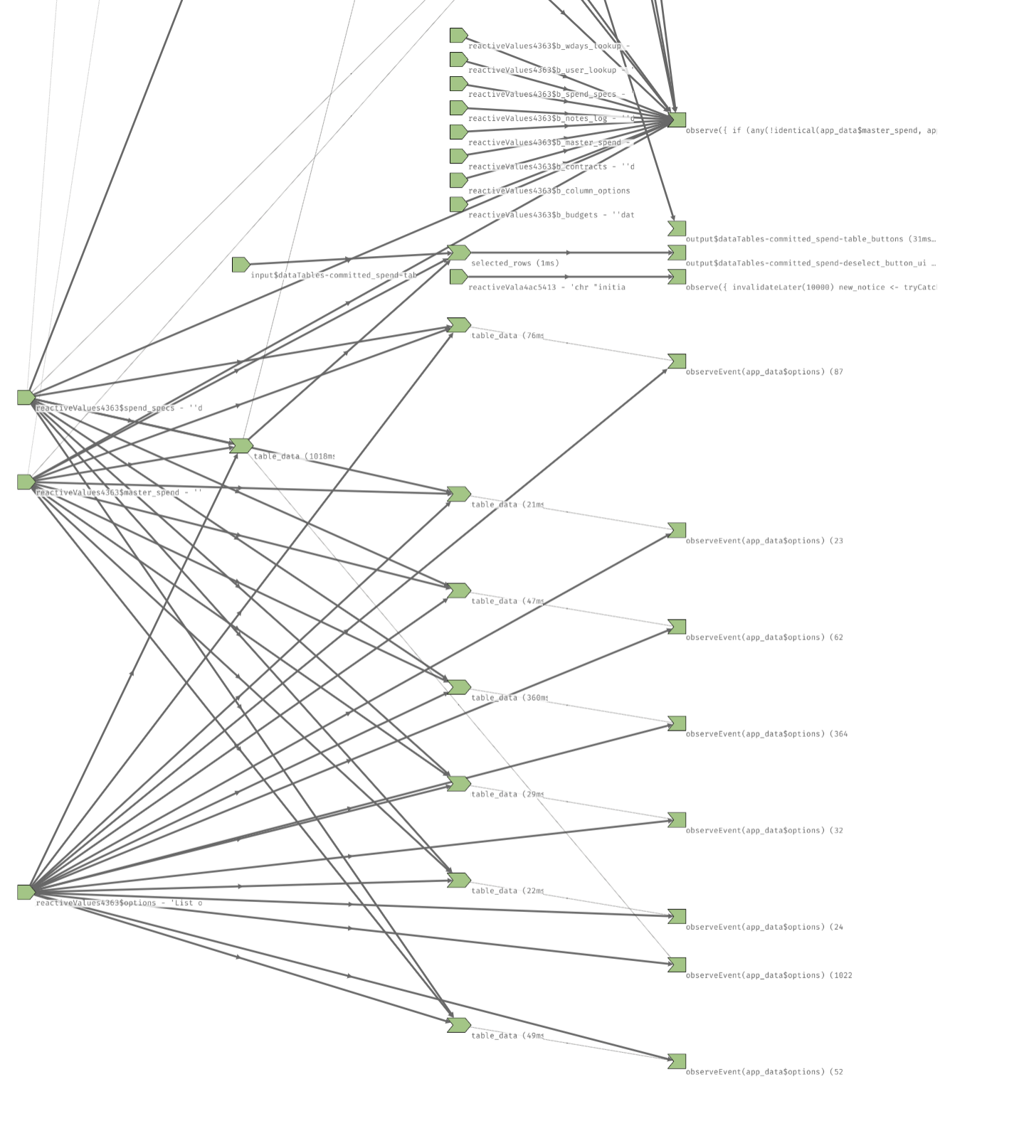
As mentioned above, this is a simple example and the image below shows what one small part of the reactlog looks like for a far more complex app. It is these situations that reactlog was designed for, to allow you to reason about what is happening at each stage of the reactive graph in your app.
Laziness FTW
The boxes on the left gives one way to understand reactivity. Another important concept which may help to contextualise the process is to realise that shiny apps use declarative rather than imperative programming.
-
Imperative programming
means that you tell the code to do something and it does it. For example when you
run
print('Hello, world')you are issuing a specific command that is carried out immediately. - Declarative programming on the other hand, involves specifying constraints and more high-level 'recipes' for how to do something, and then relying on something or someone else to decide when to translate that into action.
When we create an output in shiny, for example using a render*() function, we are not issuing a command that is carried out immediately. We are creating a 'recipe' that tells shiny 'this is how you create this output'. That recipe may be followed once, twice, many times or even never. The point is, we leave it up to shiny to decide when and how to do this.
The benefit of using declarative programming is that shiny can be as lazy as possible and only calculate something if and when it is required. You can see this in action in the example app below:
library(shiny)
ui <- fluidPage(
textInput('first_name', 'Your name:'),
textOutput('my_name')
)
server <- function(input, output) {
output$myname <- renderText({
print('This is executing now')
paste0('My name is ', input$first_name)
})
}
shinyApp(ui, server)
Note that there is a typo, the output is called 'myname' in the server instead of 'my_name'. This means that the code in the renderText() call is never run. You can verify this because you will see no 'This is executing now's in the R console either.
Now try fixing the typo and changing it to 'my_name'. You will see that it works as expected now and every time you type a name, the print statement is executing and the text output changes correctly. Note that the renderText code is not run every time you type a letter - which is what we'd expect based on everything we learned in the '4 Maxims' box. This is by design and another example of how shiny uses laziness to improve efficiency (more on this in the next tab 'Controlling reactivity').
Another example of designed laziness lies in a key part of shiny that often surprises people but works extremely well. It is often overlooked that shiny won't calculate an observer if it is not visible. This means that, by default, if your app has multiple tabs then shiny will only 'flush' the outputs on the currently visible tab.
This drastically improves the speed of shiny apps, as there may be situations where a tab has an extremely long running output which is invlidated often, but if it is never viewed then it will never be calculated - meaning the rest of the app can run much faster. Note that this function of reactivity is not visualised in the animation below, but can easily be conceptualised as follows: at the calculation stage (e.g. Step 2) if the output G is on a hidden tab, it simply won't calculate and shiny will move on to the next output. This also means that any reactive expressions which are only used in G (i.e. F) won't be calculated either. You can see how - in a large, complex shiny app - this would make a huge difference.
One consequence of this designed laziness is that reactive dependencies are dynamic . In other words, shiny tries to minimise unnecessary dependencies by working out the minimum number of times it can get away with recalculating something.
Consider the two observe() calls below:
observe({
if (input$a > 1) {
print(input$a + 5)
} else {
print(input$b)
}
})
observe({
a <- input$a
b <- input$b
if (a > 1) {
print(a + 5)
} else {
print(b)
}
})
While these observers look equivalent, there is a subtle but important difference. The second observer will always depend on both input$a and input$b, whereas the first observer will only depend on input$b if input$a <= 1. Consider the situation where input$a is set to 5 and then input$b is changed multiple times. The second observer will recalculate (the same value) several times, because it depends on input$b, whereas the first observer will not have registered the dependency on input$b because the value of input$a is greater than one. This means that the first observer will not recalculate unnecessarily if input$b is changed multiple times and will only recalculate when input$a is changed. If input$a is changed to 0, then a dependency on input$b will be created. This rendering of reactive dependencies on the fly is an important design feature as it allows even more laziness and improves shiny's efficiency drastically. Understanding this feature can make a big difference in speeding up your own apps, if you try to ensure that dependencies are only established when they are needed.
Graphing It
Reactive dependencies are dynamic (see box 'Laziness FTW'), but what are reactive dependencies? Well they are more or less what it says on the tin - if you have a variable or object which depends on a reactive value, it has a reactive dependency on that value. Take the below example:
output$my_plot <- renderPlot({
plot(runif(input$number_of_points))
})
The my_plot output has a reactive dependency on input$number_of_points. If input$number_of_points changes, my_plot will have be to re-built
Visualising how reactive objects and observers interact can help improve our understanding of reactivity in a shiny app, as well as provide a method for debugging reactivity. Consider the following trivial app:
library(shiny)

ui <- fluidPage(
    numericInput('a', 'A', 1),
    numericInput('b', 'B', 1),
    numericInput('c', 'C', 1),
    textOutput('g'),
    textOutput('h')
)

server <- function(input, output) {

    d <- reactive({ input$a + input$b })
    e <- reactive({ input$b * 2 })
    f <- reactive({ input$c * 3 })

    output$g <- renderText({ paste0('A + B is ', d()) })
    output$h <- renderText({ paste0('(2*B) + (3*C) is ', e() + f()) })
}

shinyApp(ui, server)

Copy the code and run the app yourself to get an idea of what is going on. There are three reactive values (A, B and C), three reactive expressions/ conductors (D, E and F), and two observers (G and H). If you are unsure on the difference between these three types of object, or what reactive() does exactly, take a look at the 'reactive() vs observe()' box in the 'Using reactivity' tab for more information.
We can plot the reactive dependencies of our objects, in order to better understand our app and how shiny monitors each of these. The reactlog package was designed to do exactly this (see the box 'reactlog').
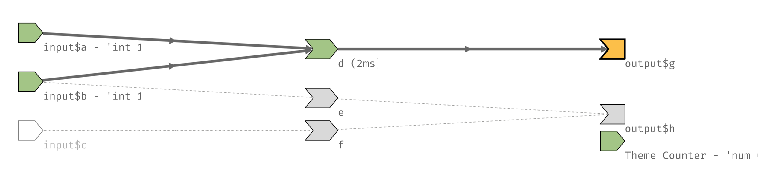
The animation below shows what the reactive graph might look like when the graph is first initiated, and then the user changes the input 'B'. See this RStudio article, which heavily inspired the animation below.
Click through the steps or click 'Play all' to cycle through the animations. The colour of a node represents its internal state: green = value is known/calculated; orange = value is calculating; grey = value is invalidated (not calculated)
Summary
So in summary:
- R does not work on a push basis, so shiny reactivity works by frequently checking whether or not something has happened and recalculating if it has.
- shiny uses an alert system where reactive objects are invalidated (indicating they have changed), which triggers a flush (recalculation) of reactive values.
- Laziness is a key part of shiny's reactivity - it will figure out how to do the minimum amount of calculation possible.
- The reactive graph is how shiny knows what needs to be recalculated in a flush, reactive contexts (dependencies) are established between various reactive elements of an app.
- You can debug reactivity in your own apps by visualising the reactive graph, using the reactlog package.
Using Reactivity
Values, Expressions & Observers
So far, in 'Understanding Reactivity' we gave a high-level overview of how reactivity works and the reactive graph. We spoke about reactive values and observers but did not go into any real detail about what these objects are and how they differ from each other. This will be addressed here, along with a discussion of two of the most powerful functions at the core of the shiny package: reactive() and observe().
There is some overlap and potential confusion with terminology being used, so the two points below will hopefully clarify what exactly these reactive objects are.
-
All objects involved in reactivity are either reactive values, expressions or observers
- Reactive values are producers, created in response to e.g. user inputs
- Observers are consumers, which take in reactive values and provide some side effect (e.g. producing plots)
- The render*() functions are a special type of observer.
- Reactive expressions are both consumers and producers (or alternatively, they are 'conductors'). They take in reactive values, transform them in some way and then pass a reactive value on to other consumers. This is usually via a call to reactive().
-
As with most of the important elements of shiny, these are all implementations of R6 classes, which means they have
reference semantics.
- Most objects in R have copy-on-modify semantics, which means that as soon as you modify a copy of a value, a new value is created in memory. We saw this in the previous tab (box 'Push or Pull?'). Consider the following example
a <- 2 # point 'a' at a value (2) b <- a # point 'b' to the same place as 'a' (the value of 2) b <- 4 # on modification the value is copied and then changed (to 4), 'b' now points at the new value so 'a' isn't affected print(a) # 2 - R6 classes use reference semantics, which means that the example above would now be (if R objects used reference semantics):
a <- 2 # point 'a' at a value (2)
b <- a # point 'b' to the same place as 'a' (the value of 2)
b <- 4 # with reference semantics, b just updates the value it is pointing at (i.e. the same value 'a' is also pointing at)
print(a) # 4
Reactive Values
Reactive values are pretty much what you'd expect from the name: values which can change over the course of a users interaction with an app.
There are two types of reactive value:
-
A single reactive value, created by
reactiveVal() -
A list of reactive values, created by
reactiveValues()
x <- reactiveVal('something')
x('something else') # call like a function with single argument to set new value
x() # call like a function without any arguments to get its value
y <- reactiveValues(x = 'something')
# get and set reactiveValues like you would a list
y$x <- 10
y[['x']] <- 20
y$x
y[['x']]
# note that unlike a list, you cannot use single-bracket indexing for reactiveValues
Despite this difference in interface, they behave exactly the same and can be used interchangeably.
Most reactive values will come from the 'input' argument, which is essentially a reactiveValues list, with one key difference - it is read-only. The values in 'input' come from user interactions and so you cannot assign directly e.g.
input$my_text <- 'hello to you too'
will cause an app to fail.
Reactive Expressions
Reactive expressions are those created with
reactive()
and have some important
properties which are covered in more detail on the right.
Conceptually, a reactive expressions can be thought of as a recipe for how to calculate a variable. The code below tells shiny that 'the variable my_data can be created by taking the first n rows of the iris dataset and appending the last m rows'. In this example, you can imagine that n and m will be numeric inputs that the user can determine.
my_data <- reactive({
rbind(head(iris, input$n), tail(iris, input$m))
})
shiny will then identify which reactive values are needed for the recipe (n and m) and try its best to calculate that variable only as much as it absolutely needs to (see 'Understanding reactivity').
Reactive expressions are accessed in the same way as reactiveVal's are, by calling
the expression as a function with no arguments. They cannot have their value be assigned because that would defeat the point
of having a recipe.
my_data()
Observers
Observers are 'terminal nodes' in the reactive graph, meaning they do not return a value (it is explicitly ignored) and instead have some sort of side effect that alters the state of the app.
Observers run when they are created (i.e. when the app starts), so that shiny can determine its reactive dependencies. They are then executed every time any of their dependencies are invalidated.
All observers are powered by the same function: observe().
y <- reactiveVal(1)
# no return value so not assigned to anything
observe({
message('the value of y is', y())
})
y(10)
Outputs are a special type of observer, with two special properties:
-
They are assigned to the 'output' object (e.g.
output$my_plot <- ...) - They have some ability to know whether they are visible or not (so they do not need to recalculate unless they are visible (i.e. on the currently selected tab).
One very important point to note about observers is that
observe()
doesn't
do
something, it
creates
something. You can see this in action if you run the following code:
y <- reactiveVal(2)
observe({
message('the value of y is ', y())
observe({message('the value of y in here is', y())})
})
y(3)
y(4)
y(5)
reactive() vs observe()
The question of when to use
reactive()
and when to use
observe()
in
the process of building reactivity, is probably one of the most common obstacles when someone starts building
shiny apps. It is also perhaps one of the most common mistakes made in shiny apps, mainly because it is usually
possible
to achieve what you want to achieve with either of them, and often the two solutions will
look on the surface as if they are identical, but one of them is always the better option.
There are two important things to consider when choosing which type of expression you should use:
Eagerness
You can see in the 'Reactive Expressions' box on the left, we've said that shiny will 'try its best to calculate that variable [i.e. reactive expression] only as much as it absolutely needs to'. You can also see in the 'Observers' box that observers will execute any time any of their dependencies are invalidated. These two sentences give you the first major distinction between reactive() and observe() - eagerness.
Reactive expressions, as mentioned, are recipes for how to calculate a variable and shiny will try to execute that recipe as little as possible - they are 'lazy'. This means that if you create a reactive() and never call it from anywhere, the code inside it will never be run. It also means that shiny will determine the fewest dependencies possible, take the following example:
a <- reactiveVal(4)
b <- reactiveVal(10)
c <- reactive({
if (a() <= 5) {
message('a is less than 5 and it is ', a())
} else {
message('a is more than 5 and b is ', b())
}
})
c() # a is less than 5 and it is 4
a(3)
# Now if we call c, it sees that a has changed so knows it needs to recalculate
c() # a is less than 5 and it is 3
# But it doesn't bother 'seeing' anything else it does not know if b changes
b(12)
c() # Note there is no output because it thinks nothing has changed
The example above integrates a second important distinction between reactive() and observe(), which is closely related to eagerness but slightly separate, and that is caching.
In short, reactive() expressions are cached whereas observers do not return a value and so cannot be cached. What this means in practice is, if none of the dependencies (that shiny detects) of a reactive expression have changed, then the same value is returned and the code does not need to be run. The example above shows why this is important to know and is a perfect example of why reactive expressions should never be used to perform side effects (see below).
Side effects
The other important consideration when choosing between
reactive()
and
observe()
is that of side effects.
There are two types of function in R, those that have side effects and those that don't. A side effect is anything that anything that affects the world outside of the function (besides returning a value). So for example:
mean(c(1,2,3)) # no side effect, simply returns a value
write.csv(iris, 'iris.csv') # side effect of writing/creating a csv file
function(a, b) {
print('calculating') # this is a side effect!
return(a+b)
}
observe()
expressions
cannot be called
and
do not return a value.
This means they are called explicitly for their side
effects.
reactive()
expressions, on the other hand,
cannot be called
and
do return a value.
This, combined with
the point on Eagerness above, indicates why you
should never use reactive() to implement a side effect
The question of which of the two to use can be nicely boiled down to the following (courtesy of Joe Cheng):
-
reactive()is for calculating values, without side effects. -
observe()is for performing actions, with side effects.
Summary
So in summary:
- Reactive values, expressions and observers are the building blocks of all reactivity
- These elements use reference semantics, rather than R's default copy-on-modify semantics
- Use reactive() to calculate values, prepare a dataframe, transform a variable
- Use observe() to create outputs, alter an existing object, make sure something executes
Controlling Reactivity
Stop...reactive time
Now that the previous two tabs have given a foundational understanding of what reactivity is and the key elements involved in making it possible, this tab will cover what to do when you want to control how reactivity works in your apps.
The first and most obvious thing to do to control reactivity is to stop it happening. There are several situations where you may want to do this, the most common being when you want to use several reactive values in a reactive calculation, but you only want to calculate them when one specific thing happens (e.g. a button gets pressed). In this situation, you would use a variation on reactive() or observe(), namely:
-
eventReactive()
or
-
observeEvent()
These both rely on another function, which is the key to stopping reactivity, and that is: isolate().
What
isolate()
does, is tell shiny 'I know this variable is reactive, but pretend it isn't'. So when the reactive
graph is formed and shiny works out dependencies, it will simply treat the reactive variable as a fixed variable and
there will be no reactive dependencies. Consider the example below:
x <- reactiveVal(1)
y <- reactiveVal(4)
observe({
message('x is ', x(), ', and y is ', y())
})
observe({
message('(isolating y)...x is ', x(), ' and y is ', isolate(y()))
})
x(3) # both observers will run
y(3) # only the first observer will run
Using isolate() removes the dependency for the second observer on 'y'.
Going back to observeEvent and eventReactive, they can both be used in the following way:
function({trigger}, {response})
With everything in the response being wrapped in isolate(), so the observer or reactive expression will only take dependencies on the contents of the trigger. This means that the following two observers are exactly identical:
a <- reactiveVal(1)
b <- reactiveVal(2)
observe({
a()
print(isolate(b()))
})
observeEvent(a(), {
print(b())
)}
Or more generally...
observeEvent(x, y)
# is exactly equivalent to
observe({
x
isolate(y)
})
# and
z <- eventReactive(x, y)
# is exactly equivalent to
z <- reactive({
x
isolate(y)
})
Its all about timing
The second way in which we might want to control reactivity more finely is to have something happen on a time-based cue rather than a user-action cue. There are two functions which can be extremely useful in this situation.
The function which will be of most use to the majority of shiny app developers is invalidateLater(), which can be placed inside a reactive expression to tell shiny to execute something after a certain time delay.
Consider the example below, where the value of x will be printed every 2 seconds:
x <- reactiveVal(2)
observe({
invalidateLater(2000)
print(isolate(x())) # using isolate() means this observer won't execute when x changes
})
This can be used for example to monitor something within your app, checking every 5-10 seconds whether a condition has been met or not.
One thing to be wary of with invalidateLater is that if the expression within is too long, it will affect your app as the calculation - just like any other reactive calculation - will stop shiny being able to calculate anything else while it is running.
If we think about use-cases for the invalidateLater() function, one obvious situation that comes to mind is that of a 'live' dataset. If we have an app that is pointed at a dataset which changes frequently, we may want to check every x minutes whether it has changed and bring in the new dataset if it has.
We can use invalidateLater() to solve this problem, but there is a major downside to this. As I mentioned before, when shiny is performing
an operation it (generally) cannot do anything else at the same time. If you are reading in a large dataset every few minutes this can have
a significant impact on your app's performance. Luckily, there is another function which can help:
reactivePoll()
reactivePoll()
works in a very similiar way to an observe(invalidateLater()) combination, but instead of taking just one
expression to execute every x seconds, it takes two functions. The first is a 'checking' function which is run every x seconds, the second
is the 'value' function, which is only executed if the checking function indicates something has changed.
What this means is, if you were looking a large, frequently-changing SQL table, you could use something like the example below:
mydata <- reactivePoll(
5000, # check every five seconds
checkFunc = function() {
dbGetQuery(conn, 'SELECT MAX(time_updated) FROM myschema.mydata')
},
valueFunc = function() {
dbGetQuery(conn, 'SELECT * FROM myschema.mydata')
})
The example above creates a reactive dataset that will check every five seconds whether the most recent 'time_updated' has changed, and if it has changed then it will read in every row from the SQL table. In this example, you can use mydata() like you would any other reactive expression and be sure that the data you are seeing is never more than 5 seconds out of date.
Hold and Give (but do it at the right time)
The final way in which we might want to control reactivity is to restrict it.
This can be particularly useful when you have a long-running reactive expression which is updating too frequently. Consider the following example:
library(shiny)
ui <- fluidPage(
numericInput('num', 'num', 5),
textOutput('slow_num')
)
server <- function(input, output) {
output$slow_num <- renderText({
Sys.sleep(2)
paste0('input$num: ', input$num)
})
}
shinyApp(ui, server)
Here a long-running expression is simulated by using
Sys.sleep
but we can see how this would cause a problem if input$num was updated
very frequently:
There are two common methods for dealing with a situation like this (and shiny provides a simple function for each): throttling and debouncing. These both work slightly differently but have the ultimate effect of restricting the number of times shiny runs the reactive expression.
Note that this is the same technique used when shiny renders value that uses a textInput, so that it doesn't re-render on every single keystroke (see 'Laziness FTW' in section 1.2)
Throttle - prioritising consistency
Throttling a reactive expression works in the following way:
- When the expression is invalidated, a timer is started for a specified amount of time (no execution takes place).
- The expression can be invalidated as many times as it needs to while the timer is counting down.
- When the timer reaches the specified time, the latest value of any reactive inputs is taken and the reactive expression is calculated.
This can be implemented as shown below (modifying our example from above):
library(shiny)
ui <- fluidPage(
numericInput('num', 'num', 5),
textOutput('throttled_num')
)
server <- function(input, output) {
throt_num <- throttle(reactive(input$num), 5000) # 5 second throttle
output$throttled_num <- renderText({
Sys.sleep(2)
paste0('Throttled input$num: ', throt_num())
})
}
shinyApp(ui, server)
and the result of this can be seen below:
Debounce - prioritising efficiency
Debouncing a reactive expression works in the following way:
- When the expression is invalidated, a timer is started for a specified amount of time (no execution takes place).
- If the expression is invalidated while the timer is running, it is started again.
- When the timer reaches the specified time without being invalidated, the latest value of any reactive inputs is taken and the reactive expression is calculated.
This can beimplemented as shown below (modifying our example from above):
library(shiny)
ui <- fluidPage(
numericInput('num', 'num', 5),
textOutput('debounced_num')
)
server <- function(input, output) {
deb_num <- debounce(reactive(input$num), 5000) # 5 second debounce
output$debounced_num <- renderText({
Sys.sleep(2)
paste0('Debounced input$num: ', deb_num())
})
}
shinyApp(ui, server)
and the result of this can be seen below:
Summary
So in summary:
- Reactivity can be stopped by telling shiny to pretend a reactive object is not reactive
- This can be done with eventReactive() and observeEvent(), which are wrappers for the crucial isolate() function
- Another way to control reactivity is by making it respond to time instead of interaction, using invalidateLater() or reactivePoll()
- You can also restrict 'overexcited' reactive expressions by using debounce() and throttle()
App Structure
Disclaimer
This tab will give you some ideas and tips on how to structure an R Shiny app. The suggestions here are not absolute rules and the approach outlined is an opinionated one - feel free to pick the bits you like and ignore the bits you don't.
Some key aspects of this structure have been chosen specifically with a complex shiny project in mind, so if you are only building a very simple app many of the suggestions may not apply. That said, it won't hurt to follow the guidelines here so that you are well prepared if your project does grow unexpectedly (as they often tend to!).
This tab will make reference to shiny modules as they are an important part of the recommended workflow set out in the following two tabs. See section 1.6 for more info about them if you aren't familiar.
The package containing this very app follows the framework set out in this tab and the following one. Feel free to check out the code to see an example of it in action!
Package it up
The first piece of advice is: structure your project as an R package. There are many reasons for doing this, namely:
- A logical folder structure and separation of R code from other objects
- Easier management of dependencies and sharing your app
- Forces you to make everything a function, which has loads of benefits, like making it easier to implement testing and QA
- Conceptually your app becomes a single contained entity rather than a project which combines a shiny app with a set of additional R scripts (a slightly more abstract point but to me this is very important!)
The best way to create an R package is beyond the scope of this app, but there are some links in the References & Further Materials section which cover creating an R package. If you're a DfE colleague, there was also previously a C&C talk covering exactly this, presented by Mr Jacob Scott (link here).
Everything has a home
Below you can see how a shiny project might be structured in practice. The text in italics gives a brief description of each element.
Blue boxes represent folders and can be clicked to expand and see contents. Black boxes represent individual files.
A rose by any other name
The naming conventions in the R/ folder above are largely inspired by those proposed in the golem R package framework. They assume that you are a) structuring your app as a package and b) are using shiny modules throughout your app.
The rules for the naming convention proposed here are as follows:
- All modules (in the case of e.g. a shiny dashboard these are likely to each correspond to a tab) are numbered in order of where they are in the app and given a short name. For example, if the first tab in your app is an info tab, you would define the module UI and server in the 'mod_01_info.R' script.
- All functions are defined in scripts which are named for the module the function is used in. For example, if in your info module, you have a series of functions for importing data, these would be defined in 'mod_01_info_fct_importData.R'. This makes it immediately clear that the script contains functions for importing data and that those functions are used in the info module.
- Any functions which are either not used in a module, or are used in multiple modules and it doesn't make sense to associate them with a single module, can use the same naming conventions but without the module prefix. For example, if the import data functions from above where used in various modules they could be kept in a script named 'fct_importData.R' instead.
- Any utility functions (simple/helper functions that do not perform important business logic and are potentially optional) go in scripts prefixed with 'utils_'. For example, you may have some functions for formatting text like e.g. as_money(). These could go in utils_formatting.R.
- Your app UI and app server go in app_ui.R and app_server.R respectively.
To see this in action, you can view the source code for this very package. As mentioned in the disclaimer above, this is just one opinionated way of structuring and naming an app, so feel free to take what works for you and ignore what doesn't. What is most important is that others can understand your structure and easily navigate your code.
DfE-Specific
There are a few final points to bear in mind if you are a DfE colleague and the app you are developing as a package is to be deployed to our internal RStudio Connect servers.
Deployment Pipeline
Our deployment pipeline determines the content you are deploying based on the contents of your project. This
means that if your root folder doesn't contain either an app.R file or ui.R & server.R files, the deployment
will fail as it will not recognise that you are deploying a shiny app. To get around this, include an app.R
file that calls a function from your package. This function must return a shiny app as an object. The easiest
way to do this is to use
shiny::shinyAppDir()
in your run_app() function, so it might look
like this:
run_app <- function() {
if (interactive()) {
# interactive()=TRUE when function is run from the console
shiny::runApp(appDir = system.file('app', package = 'myPackage'))
} else {
# interactive()=FALSE when being sourced (i.e. when deployed)
shiny::shinyAppDir(appDir = system.file('app', package = 'myPackage'))
}
}
and your app.R file should look like this:
pkgload::load_all() # roughly equivalent to library(myPackage)
myPackage::run_app()
Dependencies
As with any app that is deployed to our RSConnect servers, it must be dependency-managed using
renv
. Contrastingly,
R packages manage dependencies using roxygen documentation and a DESCRIPTION file.
This can cause some confusion and issues when deploying apps to RSConnect, but as long as you keep on top of both methods you should be fine. When you want to use a package in your app's functions, you must:
- Import that package somewhere in your roxygen comments with @import, @importFrom or @rawNamespace, and/or specify it in your code directly with [package]::
- Add the package to your package's DESCRIPTION file, under Depends or Imports
- Run devtools::document()
- Add the package to your renv lockfile (i.e by installing the package and running renv::snapshot()
Sharing is caring
As has been mentioned elsewhere on this tab, it is highly recommended that you use shiny modules to partition your app into logical, manageable chunks. This is covered in more detail in the next tab, but for those who already know about modules and have used them before, this box will cover something that can cause issues if you don't have a plan in place to deal with it - sharing data between modules. This is being addressed here because although it largely relates to modules, it is a design choice to be made when structuring your app and the method proposed here is again opinionated so feel free to ignore it or come up with your own solution.
If you have not used modules before, check the next section and then return here!
Sharing data between modules can become tricky when working with reactive values, because although you can pass reactive arguments to modules and return reactive objects, it quickly becomes difficult to understand how and why values are updating in some modules and not others.
The solution proposed here makes use of the fact that a) reactiveValues() lists are R6 objects and b) this means they use reference semantics and are not copy-on-modify.
What this means is that when you create a reactiveValues list and then pass it as an argument to a module, the module simply receives a pointer to that reactive list in memory, rather than a separate copy of it. So if you have a single reactiveValues list with all your important app data in, you can just pass this list to each module and they will all be immediately aware of changes to the list, regardless of where the change originates from.
In practice, I would suggest you always specify a reactiveValues list called e.g. app_data in your app server function, and then pass it as an argument to each module. This list can then be used to store anything which might be required by multiple modules e.g. datasets, information about the user/session, theme/colour options that the user can change etc.
Summary
So in summary:
- Structure your app as an R package
- Use shiny modules (see next tab)
- Use a consistent naming convention that distinguishes between the different core components of your app
- Use reactiveValues to share data between modules
Shiny Modules
Why...so...modular?
This tab will introduce Shiny modules and discuss how and why you might use them. If you are developing a shiny app which you think could potentially grow in future or be anything more than a very simple app, you should absolutely, definitely use modules. There are two key benefits to using Shiny modules and they are outlined below:
- If you've ever built a complex shiny app you'll know it can easily reach thousands of lines of code if you aren't careful. This quickly becomes a nightmare to maintain and debug, as you can end up scrawling through lines of your server to find where that one reactive object is defined. Modules give you an easy way to split your app code into separate, manageable scripts.
- The '1000 button problem': usually if you find yourself repeating code, you should be writing a function and calling that instead. This isn't so straightforward with reactive Shiny code because of namespacing. Every instance of an object needs a unique ID to match the UI to the server and this can quickly cause major headaches when developing your app. Modules provide a neat way to resolve this.
From personal experience, the first of these is the more useful aspect of Shiny modules and the reason why I would recommend always using them unless you have a reason not to.
The box on the right shows an example of how modules can be used, so feel free to use this as a starting point for developing your own modules.
On a side note: be careful when researching/googling shiny modules and be sure not to confuse them with wahani modules, which are an unrelated topic in R.Housekeeping
As mentioned above, one of the key benefits of using shiny modules is keeping different elements of your app separate and in short, manageable scripts. The workflow proposed here (in this tab and the previous tab) is inspired by various other frameworks and is opinionated. As always, feel free to pick and choose which of the below you use, but when it comes to using modules, the following points are recommended:
- Each page of your app should be a separate module. This is straightforward for dashboard-style apps where you can simply have a separate module for each tab, for other apps you may have to make judgement calls about the separate parts of your app.
- Each module (UI and server function) should be in its own script, named according to the conventions outlined on the previous tab (e.g. 'mod_01_homepage.R').
- Every page's module server function should have a mandatory data argument, to which can be passed your app_data reactiveValues (see the 'Sharing is caring' box on the previous tab).
- Each module function should be documented in the same way as a normal function with roxygen comments.
Following these steps, as well as following the advice to structure your app as a package, will also mean that you can reuse modules in different apps. You could even develop a package with a module in and then just use that package when you are developing other apps in future. For example, if you have a particular section of reactive UI that is used in multiple apps.
Summary
So in summary:
- Always use modules!
- Separate your app into sections and have each section in a separate
- Use modules as an alternative to functions which have reactive inputs and outputs
- Shiny modules are an implementation of the software development method of namespacing
1000 Button Problem
Imagine you are building an app with several independent counter buttons. This can be achieved using functions for UI and server logic, but for a very large app you would run into problems due to the fact that input and output IDs share a global namespace in shiny. This means that all inputs and outputs must have unique IDs.
This issue is resolved in computer science by using namespacing whereby objects must only have unique IDs within their namespace and namespaces can be nested. In practice you can simply think of a namespace as a prefix to an ID. For example, if you have two outputs called 'my_button', you can put them into separate namespaces called 'first' and 'second'. This would be equivalent to (but far more elegant than) renaming the outputs 'first-my_button' and 'second-my_button'.
Shiny modules were introduced to allow developers to take advantage of namespacing. See below for how to use them, in the context of an app with multiple counters.
library(shiny)
counterButton <- function(id, label = 'Counter') {
ns <- NS(id)
tagList(
actionButton(ns('button'), label = label),
verbatimTextOutput(ns('out'))
)
}
counterServer <- function(id) {
moduleServer(
id,
function(input, output, session) {
count <- reactiveVal(0)
observeEvent(input$button, {
count(count() + 1)
})
output$out <- renderText({
count()
})
count
}
)
}
ui <- fluidPage(
counterButton('counter1', 'Counter #1'),
counterButton('counter2', 'Counter #2'),
counterButton('counter3', 'Counter #3')
)
server <- function(input, output, session) {
counterServer('counter1')
counterServer('counter2')
counterServer('counter3')
}
shinyApp(ui, server)
There are 5 important points to note about the code above:
- The module is defined in two parts just like a shiny app, with a UI and a server function
- Both elements of a module take in an id argument. This is crucial as it allows shiny to match the module UI to module server for each instance of the module.
-
The UI function uses a function from shiny to access the current namespace.
NS(id)will return a function that adds the current (unique) namespace to whatever is supplied to it. So by applying the resulting ns() function to each output in the module, the outputs will be unique to that particular 'id'. - Note the moduleServer call in the counterServer function. This allows you to write code as you would for a shiny server, using the input, output and session objects as required.
-
Outputs in the server function do not need to be wrapped in a namespacing function because this is handled
by moduleServer(),
but if you use renderUI(), any outputs or inputs must be namespaced in the same way as in the UI
function.
This is done by adding the following line of code to the top of your moduleServer function call:
ns <- session$ns
Using CSS
What is CSS?
In Section 1.1 'What is shiny, actually?', I described shiny as 'an R to {HTML-Javascript-CSS} translator', as these are the three core components of the front-end of most modern web apps. One way to decribe this triad is: HTML (HyperText Markup Language) provides the building blocks for your UI; Javascript determines what the building blocks do and CSS (Cascading Style Sheets) determines what the blocks look like. This is perhaps an oversimplification (disclaimer: I am not a front-end dev or web designer!), but I think it gives a good practical understanding of how the three interact.
In shiny, the HTML code will mostly be generated using shiny functions such as
fluidPage()
p()
and the various
*input()
and
render*()
functions.
The javascript in the app comes from many places, including the shiny package itself and this is discussed in detail in other tabs. The CSS that comes bundled with shiny gives a generic, bland look and feel to the app so in order to spice things up, you must add your own CSS.
CSS can be used to specify the color, shape, size, shadow, background colour, spacing, padding and many other attributes of each individual element or type of element on your page.
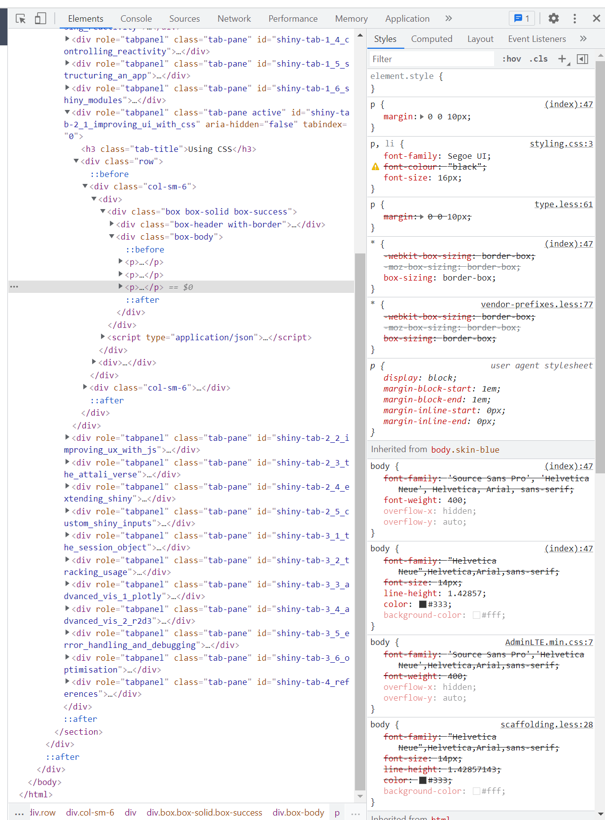
You can see some examples of CSS if you inspect any web app - including this one - by opening the developer tools (usually by right clicking and 'Inspect'). The picture below shows an example of what you might see:
The pane on the left shows the HTML of the page and the pane on the right shows some of the styles specified by the CSS of the page.
{shinydashboard(Plus)} vs {bslib}/{thematic}
Note: this box is not technically about CSS but what is discussed below is an important design choice for the developer of a shiny app (as is CSS).
When deciding what your app will look like, CSS gives you fine-tuned control over each object in your UI. Before you reach this point though there is often a key decision to be made: to dashboard or not to dashboard.
There are essentially limitless ways to structure a shiny app, as you could always even write the custom HTML to achieve
the layout you desire, but typically (in my experience at least) it will usually boil down to whether a dashboard structure
makes sense or not. If it does, you can make use of the
shinydashboard
and
shinydashboardPlus
packages to speed up your development, if not you will probably use a vanilla shiny
fluidPage()
or
navbarPage()
layout and have more design choices to make about how to structure
pages and navigation etc.
To clarify, this advancedShiny app uses a dashboard layout - a header, a body (central pane) and a sidebar (navigation pane) which allows you to switch between different named tabs, each one containing related information in structured boxes/sections. A non-dashboard layout may consist of a single page, or multiple pages where the layout differs depending on which page is currently visible, for example.
The shinydashboard package can be used (and has been used here) to get a dashboard-style look and feel to the app, providing
functions for
dashboardPage()
dashboardHeader()
dashboardBody()
etc. Additionally
the
shinydashboardPlus
package extends this and gives more options such as closable and collapsible boxes,
and more colours to use.
If your app is not a dashboard layout, you can make use of the
bslib
package which allows you to specify
custom theming and use existing Bootstrap themes in your app.
bslib
also makes it possible to use Bootstrap
4 or 5, where shiny defaults to Bootstrap 3.
As
bslib
is (like shiny) an RStudio package, it benefits from seamless integration with base shiny. All
shiny's top-level layout functions (e.g. fluidPage), have a 'theme' parameter. So you can simply supply a function from bslib
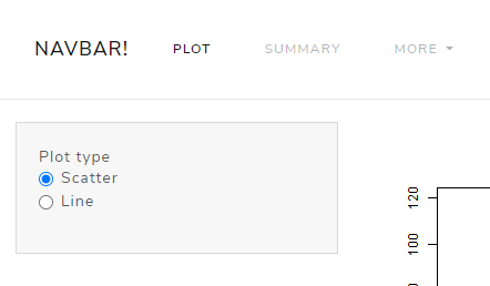
as an argument to that. Take the example app below (adapted from an RStudio example app):
library(shiny)
ui <- navbarPage('Navbar!',
tabPanel('Plot',
sidebarLayout(
sidebarPanel(
radioButtons('plotType', 'Plot type',
c('Scatter'='p', 'Line'='l')
)
),
mainPanel(
plotOutput('plot')
)
)
),
tabPanel('Summary'),
navbarMenu('More')
)
server <- function(input, output, session) {
output$plot <- renderPlot({
plot(cars, type=input$plotType)
})
}
shinyApp(ui, server)
This app has the basic shiny styling (see sample below):
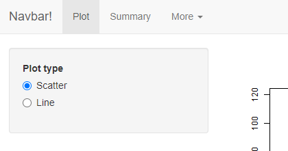
But by using
bslib
you can change the look and feel with just one line of code,
added to the
navbarPage()
call:
...
ui <- navbarPage('Navbar!',
theme = bslib::bs_theme(bootswatch = 'lux') # add theme
tabPanel('Plot',
...
Resulting in app that looks slightly more appealing:
Admittedly, in this example app the changes aren't radical (mostly just the font, some colouring and the behaviour of the navbar buttons), but for more complex apps you can see how powerful it would be to overhaul the general look and feel with a single line of code.
Additionally, you specify your own custom theme with the various arguments to
bs_theme()
as opposed to a pre-made bootswatch theme (like the example above). If you choose this route you have far
more control and can even adjust your theme using a real time editor via the
bs_themer()
function.
How to add CSS to your app
There are three main ways you can add custom styles to your app. This tutorial will not cover CSS syntax, but will assume you have a working knowledge of how to style HTML elements using CSS.
1. Separate CSS file
This is the best way to add custom CSS to your app. It involves keeping all your styling contained into a single file or collection of files, away from the logic of your app. It also makes it far easier to maintain consistent styles across your entire app. To include a file in your app, you should store it in the www/ folder (see 1.5 - Structuring an app).
Assuming you have created a CSS file called 'styles.css' and stored it in your www/ folder, you then simply need to add the following code to your UI:
tags$head(tags$link(href = 'styles.css', rel = 'stylesheet', type = 'text/css'))
This will make any styles available to your app.
Per-element styling
A quicker but far more messy way to style an element is to include it directly, using the 'style' argument to the element ( where it is available). For example, it can be used on a 'div' to style everything within it:
tags$div(
style = 'font-size:40px; font-weight:bold;',
p('This text will be large and bold')
)
Alternatively, you can include class definitions using
tags$style()
, e.g.:
tags$style('
.blue-stuff {
color: blue;
}
.red-stuff {
color: red;
}'
)
Dynamically add CSS
This is rarer and should only be used in specific cases, but the shinyjs package can be used to add a class to an object after the app has been launched. See example below (using tags$style() css from above):
ui <- fluidPage(
shinyjs::useShinyjs(),
tags$style('
.blue-stuff {
color: blue;
}
.red-stuff {
color: red;
}'
),
p('This is the text', id = 'my-text'),
actionButton('red', 'Make red'),
actionButton('blue', 'Make blue')
)
server <- function(input, output) {
observeEvent(input$red, {
shinyjs::removeClass(id = 'my-text', class = 'blue-stuff')
shinyjs::addClass(id = 'my-text', class = 'red-stuff')
})
observeEvent(input$blue, {
shinyjs::removeClass(id = 'my-text', class = 'red-stuff')
shinyjs::addClass(id = 'my-text', class = 'blue-stuff')
})
}
shinyApp(ui = ui, server = server)
Getting {sass}y
Once you have mastered adding CSS to your app, you can begin to make use of SASS (Syntactically
Awesome Style Sheets) - a CSS extension language described as 'CSS with superpowers'. All SASS is,
is a way to make managing large/complex CSS sheets easier, by adding various useful things such as:
allowing you to set variables, nest your styles and use partial styles (among other things). SASS
then generates the final CSS stylesheet automatically. Helpfully, there is an R package allowing you
to make use of SASS in your shiny apps with almost no additional effort required - the package is called
sass
View the code at the top of the app_ui() function for this package to get an idea of how to use
sass
in this proposed workflow.
Using Javascript
What is Javascript?
As mentioned in tab 1.1 ('What is shiny, actually?'), Javascript is one of the three languages of the web that shiny code gets converted into. The way I like to think about it is that Javascript handles how objects move and interact with the user. In reality, Javascript is a very powerful programming language that can be used in a plethora of ways.
As has already been stated by others before me, Javascript really is the best way you can take your Shiny skills from decent to world-class. Proper use of Javascript is, in my opinion, the number one way to improve user experience in your app. When it comes down to it, user experience is almost always the one key metric for how successful an app is. If a user can't get what they need from an app or faces unnecessary complications and hurdles to doing so, it doesn't matter how pretty it looks or how many complicated concepts it implements, they simply won't use it.
Javascript is more complicated than its two companions in shiny web development (HTML and CSS), but is far more powerful as a result. Many of the core concepts of Javascript have parallels in R - or most other programming languages for that matter (variables, functions, conditionals etc.).
This tab will not discuss the technicalities of using Javascript in any depth, as there are already fantastic resources available elsewhere:
- See here for a basic introduction to Javascript.
- See here for a slightly more in-depth tutorial.
- See here for a more detailed discussion of how to use JS in production shiny apps.
Instead, this tab will focus on trying to explain practically why you might want to look into using JS or ways to get started.
Some cool use cases for adding JS to your app
This is just some of the ways I've used Javascript in an app or you might want to (this list is far from exhaustive):
- To monitor whether a user makes changes so that when they try to close the app they get a popup saying 'you have unsaved changes'
- To animate an element of the page when a user hovers their mouse over it
-
To speed up the reactivity of your UI using e.g.
shinyjs -
To create custom interactive, animated graphics using e.g.
r2d3 - To insert a custom API into your app to allow communication with other programs/services
- To identify a user's browser information to enable customise your app based on viewing device
How to add javascript to your app
As with CSS, there are two main ways to add JS to your app: the clean way and the messy way.
The messy way
Javascript code can be added directly inline to your app, using
shiny::JS()
or
tags$script('{javascript code}')
The clean way
You can keep your Javascript code in a separate file(s) in the www/ folder and include them using
shiny::includeScript()
or
tags$link(src = 'myscript.js')
shinyjs
One of the best ways to get started using Javascript in your shiny apps is to leverage the powerful and lightweight
shinyjs
package. Created byDean Attali, it wraps several useful Javascript
actions into neat R functions. This allows you to introduce Javascript functionality to your app without even having to learn the language
to begin with!
For a full list of what shinyjs provides, see the documentation site but see below just a couple of examples.
Hiding/disabling elements
This is probably what I use shinyjs for the most, quickly and easily hiding, unhiding and disabling elements. There are many situations
where you want to take the ability to do something out of your users' hands for a period of time. The shinyjs functions make this very easy.
See an example below. Notice the use of
hidden()
to ensure the element starts in a hidden state - there is an equivalent
disabled
function too for starting an element in a disabled state.
library(shiny)
library(shinyjs)
ui <- fluidPage(
useShinyjs(),
hidden(p('some sample text', id = 'txt')),
actionButton('show', 'Show text'),
actionButton('hide', 'Hide text'),
actionButton('disable', 'Disable hiding/showing'),
actionButton('enable', 'Enable hiding/showing')
)
server <- function(input, output) {
observeEvent(input$show, {
show('txt')
})
observeEvent(input$hide, {
hide('txt')
})
observeEvent(input$disable, {
disable('show')
disable('hide')
})
observeEvent(input$enable, {
enable('show')
enable('hide')
})
}
shinyApp(ui, server)
Delaying events
There are multiple ways to delay reactivity in shiny (see 1.4 - Controlling reactivity), but shinyjs provides yet another way to
simply control the flow and timing of events in your app, using the
delay
function.
See an example of this below:
library(shiny)
library(shinyjs)
ui <- fluidPage(
useShinyjs(),
p('some sample text', id = 'txt'),
actionButton('hide3', 'Hide text for 3 seconds'),
actionButton('hide1', 'Wait 3 seconds, then hide text for 1 second'),
)
server <- function(input, output) {
observeEvent(input$hide3, {
hide('txt')
delay(3000, show('txt'))
})
observeEvent(input$hide1, {
delay(3000, hide('txt'))
delay(4000, show('txt')) # important: delay time is from when observer first runs
})
}
shinyApp(ui, server)
Attali-verse
Dean Attali
In the previous tab, I introduced shinyjs as one of the best ways to get started using Javascript in your shiny apps. This package was created by an R guru by the name of Dean Attali. Dean runs an R Shiny consulting firm and has created several R packages specifically to enhance shiny apps and fill some of the gaps in base shiny functionality.
This collection of packages do not have an official name so I've (semi-seriously) referred to them as the 'Attali-verse'. There are several packages, each with their own specific use case - and I personally have found some of them invaluable when creating interactive, user-friendly apps.
This tab introduces some of the most useful packages, because I believe that all shiny developers should at least be aware of them as they may make your life much, much easier.
See Dean's Github for more or to see all other packages.
shinyalert
shinycssloaders
...and the rest
Extending Shiny
Javascript is powerful
shinyHelper, shinyFeedback, shinyEffects
htmlwidgets
Higher-order reactives
Custom Shiny Inputs
What actually are shiny inputs?
Bindings and Findings
Creating your own input
{charpente}
Session Object
Apps, Clients, Servers, Sessions
Making the most of sessions
onDisconnect, userData etc.
Under the hood of the session object
DfE-Specific advice
Tracking Usage
Why might you want to track app usage?
The manual way
The shinylogs way
DfE-Specific advice
Visualisation with plotly
What is plotly? and what is Plotly? and what is {plotly}?
short version: Plotly created plotly which can be accessed via {plotly}
The full extent of interaction and customisability
{plotly} vs {ggplot2}
Some examples
Visualisation with r2d3 et al.
What is d3? and what is {r2d3}?
Complete control (examples)
{r2d3} vs {plotly} vs {ggplot2}
Other JS plotting libraries
e.g. {leaflet}, {dygraphs}, {networkD3}, {echarts4r}, {highcharter}, {sigmajs}
Error Handling & Debugging
With base R
tryCatch(), withRestarts(), stop(), warning(), message(), browser()
With {shiny}
With {testthat} and {shinytest}
With {whereami}
Optimisation
Optimising using {profvis}
Caching in shiny apps and {memoise}
Asynchronous programming with {promises} and {future}
Some common optimisations
e.g. multiple tabs, paste>sprintf, data.frame>data.table, grepl^>startsWith, vectorisation/de-looping, use SQL databases, {Rcpp}, {minifyr}